Assignment 3 - Wolf Telemetry Data

Overview

• Working with CSV Data
  • How to load csv data into GeoDatabase
  • Using Field Calculator
  • Create a Layer using XY Coordinate Pairs
• Relational Data
  • How to join data in ArcGIS Pro
• Point to Line
  • Create a transect for each wolf in the captured data
  • Calculate total length
  • Calculate avg distance traveled per day
• Create a Relational Dataset
  • Create a Domain
    • Map Health Conditions to Captured Wolf Data
• Pick a Wolf and create a map
  • Pick a single wolf that has observations
    • Create a map of its tracked locations
      • We need to show its pack boundary.
      • Label the start date of tracking.
      • Label the end date of tracking.
      • Show the telemetry layer for this wolf.
      • Show the Capture Dates Associated with this wolf.
    • Put other details needed to communicate about this wolf.
      • Create a table showing the details of the wolf
      • Answer the questions and write your answers for context about our wolf.
    • Add a legend so we know what we are looking at.

Deliverables

• Answer the following questions, and summarize the answers in a text box in our map.
  • How many other wolves and what are the names of the wolves in Boyds Pack?
  • Who is the oldest and youngest member in this pack?
  • Are there any other wolves in the pack that are collared?
  • What is the average weight, and health condition of the male wolves that have been captured and are alive in the North Washington Packs? How does this compare to Boyd?
  • For the sampled observations, how much time are the wolves spending time inside the pack boundary vs outside the pack boundary (just in terms of observations)? Do you think we need to expand the boundary based on this number?
• An exported map that relates all the data we have about Boyd

Lets Get Started

• Create a folder for this assignment. We want to be able to keep a copy of our downloaded data separate from the other stuff we will be doing.
  • Create a sub folder call Raw.
  • Download the csv files from github and save them to this folder.
• Create a new ArcGIS Pro Project, and save assignment directory.

Lets set up our ArcGIS Pro Project now.

Open Catalog and we are going to add our raw data folder as a directory that is discoverable by ArcGIS.

There will be an item called folders in Catalog, right click this folder, and click Add Folder Connection. Navigate to your raw data directory and click OK.

You can now see the csv files that we downloaded in this folder when you expand it.

Import data to geodatabase

We can work with CSV files directly since we have added a folder connection. However, I suggest that it is better to have a save a unaltered version of the raw data, and have a derivative dataset which you can mess up. That way, if you need to start over in any process, you don’t have to worry about downloading the data again.

So, lets import our csv to the geodatabase.

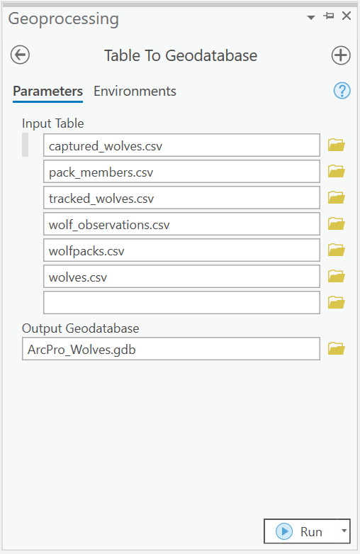
Right click the ArcGIS Pro Default Geodatabase. Go to import, and select Tables.

Use the file navigator to import all the csv files from your raw directory to the default geodatabase.

Click Ok. And the Tables should now be listed in your geodatabase, if not right click and refresh.

So what is this data?

Well, lets take a look. Each of these tables are stored as Database Tables; that is, they only are storing attribute data. Or at least thats what ArcPro thinks.

Right Click on each of the layers and select Open Table.

There sure is data in some of these tables that looks like location data though.

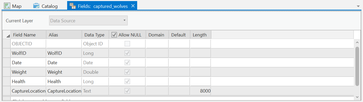
Now for each of the tables, right click and select Data Design -> Fields. This will open a new view (see below).

This option shows you all the field names, and the data type that field is storing. This is important becasue it lets us know what we can do with each of these fields and what data should be where.

If you need a refresher on field types, take a look here.

Our dataset is built to keep track of all things wolves, so we got information about wolves, wolf packs, collared and capture locations, and GPS tracks associated with a Collar.

Woof… Thats a lot to keep track of. Thankfully, we can use joins and relates to be able to help us keep track of each wolf and their associated data.

After taking a look at these data, it appears that we actually have some spatial information that we want to work with right? So lets start with that.

Field Calculator

Attribute data can also be added to our map. So starting with our captured_wolves, lets right click and select Add to Map.

In the Map Pane, lets right click, and select Open to view the attribute data.

So the CaptureLocation field. Sure looks like an geometry field to me, but as we saw its stored as a text field. For us use this data, we need to split up this field into two separate fields: a latitude, and a longitude data set.

To do so, we are going to use something called the Field Calculator.

The Field Calculator is a button at the top of the table view we opened. Click Calcuate. A new window will open.

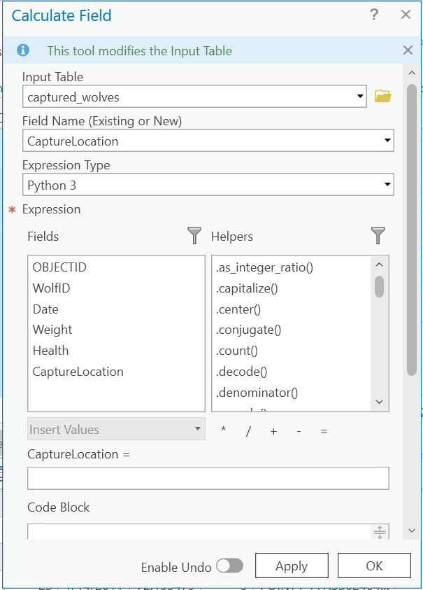
Now, we are going to add our fields with a new value.

Lets do it in three steps. Type in the following variables.

First, Create the Lat_Long field, and remove the leading Point text with the parathesis.

Input Table: Capture Wolves
Field Name: Lat_Long
Field Type: Text
Expression Type: Python3
Lat_Long = get_xy_text(!CaptureLocation!)
Code Block:

# Define a function called get_xy_text that takes a parameter "point"
def get_xy_text(point):
    # for a parameter point, replace the text 'Point', '(', and ')' with nothing. Essentially deletes them.
    point_details = point.replace('POINT ', '').replace('(', '').replace(')', '')
    # Return the variable; should be two decimal numbers separated by a space
    return point_details

Now we are going calculate the Latitude and Longitude fields.

Pay close attention to which item in the coordinates is supposed to be the x axis and which is the y axis.

Click Calculate again.

Input Table: Capture Wolves
Field Name: Latitude
Field Type: Float
Expression Type: Python3
Lat_Long = get_xy(!Lat_Long!)
Code Block:

And repeat for Longitude. You will use this same function, but you have to return the correct number for Longitude. So update the return statement to return the the x value.

# Define a function called get_xy that takes a parameter "point"
def get_xy(x_y):
    # for a parameter point,  split the text on a space. Returns a list of two objects. 
    point_details = x_y.split(' ')
    # Return the first variable in the list. A list is zero index. 
    return point_details[1]

Cool now we are getting somewhere. Lets add our points to our map now.

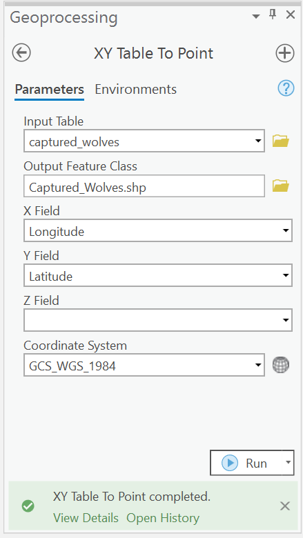
Click View in the Ribbon, and open the Geoprocessing pane by clicking the Geoprocessing button. You can search for tools here like the XY Table to Point.

Lets open our Captured Wolves table, save the layer to our geodatabase, and use the correct fields that we just calculated to use for our Longitude and Latitudes fields.

Since our data is in decimal degrees, we are using the Geographic Coordinate System WGS 1984.

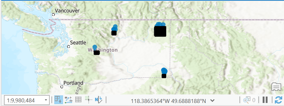
Great, We now have points on our map. Lets repeat this process for wolf observations. Not, that you will have to update which field is used when calling our function we wrote. Fields are used by calling the field name surrounded by !Location!

When you get the layer added to the map, it will look like a giant blob of data in different locations. Thats because we have logged over 155,000 locations!!!

Create a transect

Now that we have all the point locations where a wolf hase been observed, lets make lines representing the actual routes that a wolf has traveled.

Lets do some stuff to work with a managable set of data that makes sense.

Lets pick a wolf, and explore how many observations there are, and the max and min date the observations.

Say, lets choose Boyd.

Well, for us to know what Wolf ID Boyd is, we will have to join some data to our observations data.

Lets go to Catalog, and add our Wolves Table to our map.

Once added to the map, we are going to want to join our tables.

I like to always think about the cardnality of our data when choosing which layer to start with the join.

So in this instance, we would like to right click the layer with the lower cardnality. In this case, the table with the more ‘repeats’ for data is our observations.

Right click our Wolf Observation Points and select Join -> Add Join.

This will open a new window.

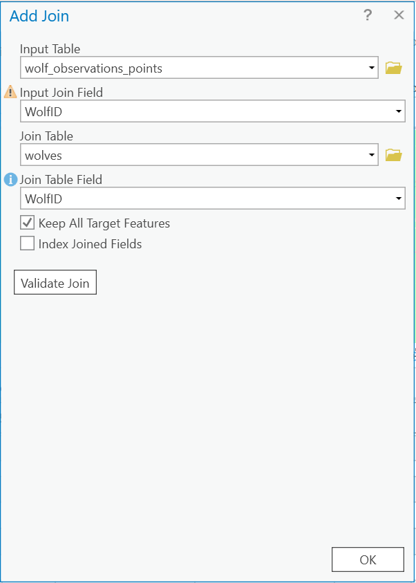
We are going to join our Wolves Table, and for these tables, our Primary Key and Foreign Key are the same; that is WolfID.

Basically, this is saying for each observation of this wolf in the observations table, go find me the correct data from the wolf table, and append it to this row.

SELECT 
    * 
FROM 
    wolf_observations_points
left join wolves on 
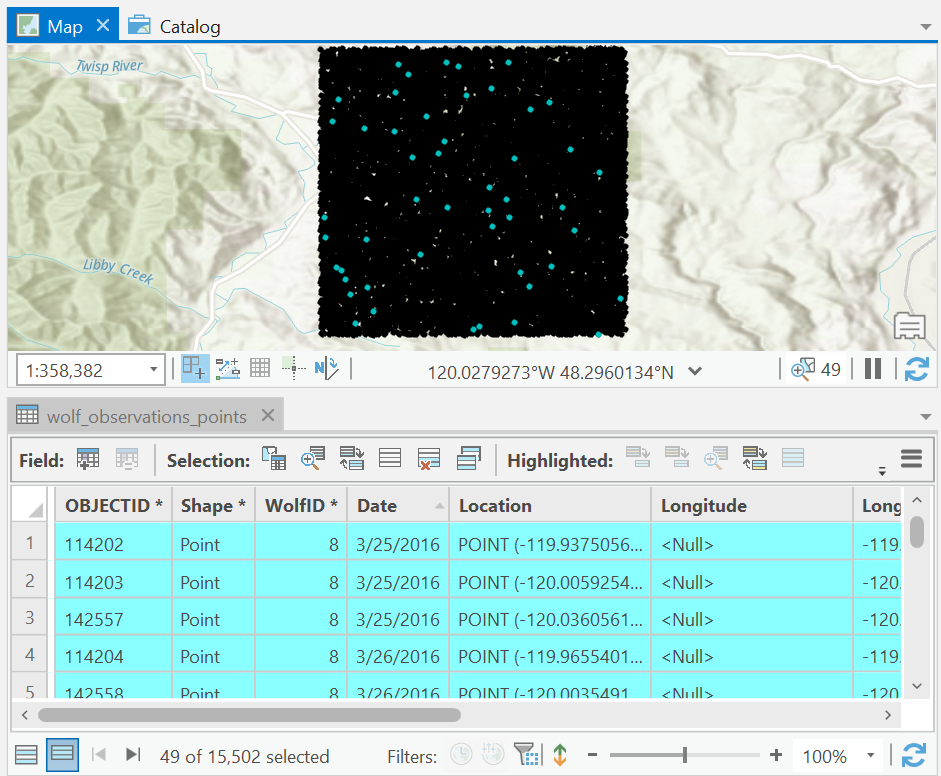
    wolf_observations_points.WolfID = wolves.WolfID

Cool, now we at least know which observations that are tied to Boyd.

So lets filter them. Lets apply a Definition Query and show only observations for Boyd.

You did this last week, so I’m going to let you take care of this.

So once you did that, you should be able to open the attribute table, and see that there are still over 15k observations.

Lets say we are tasked with providing a summary of all Boyds locations for a given week, your choice of week.

When we look at this data, we can sort by fields by double clicking the Header in the Table view of our wolf observations points data. We can see that the most recent data of observations for Boyd was 04/06/2016 and the first observations started 02/10/2008. So we have 8 years of data here!

Lets filter down this data to make it a little bit more manageable.

We are going to select rows within this two week window. Hit the Select By Attributes button, and filter the rows where the dates are for your two week observation window.

Leaving this vague here, but think about which Logical Operators you will use to get this selection.

You should get something like 50ish points from the selection.

To make this easy to present in our map, lets export this subselection to make it its own layer.

Right click on the layer, and select Data -> Export Feature.

Save to your geodatabase with a name that makes sense.

How bout.

Boyds_Observations_StartDate_to_EndDate

Of course replacing the start data and end date with the dates you chose accordingly.

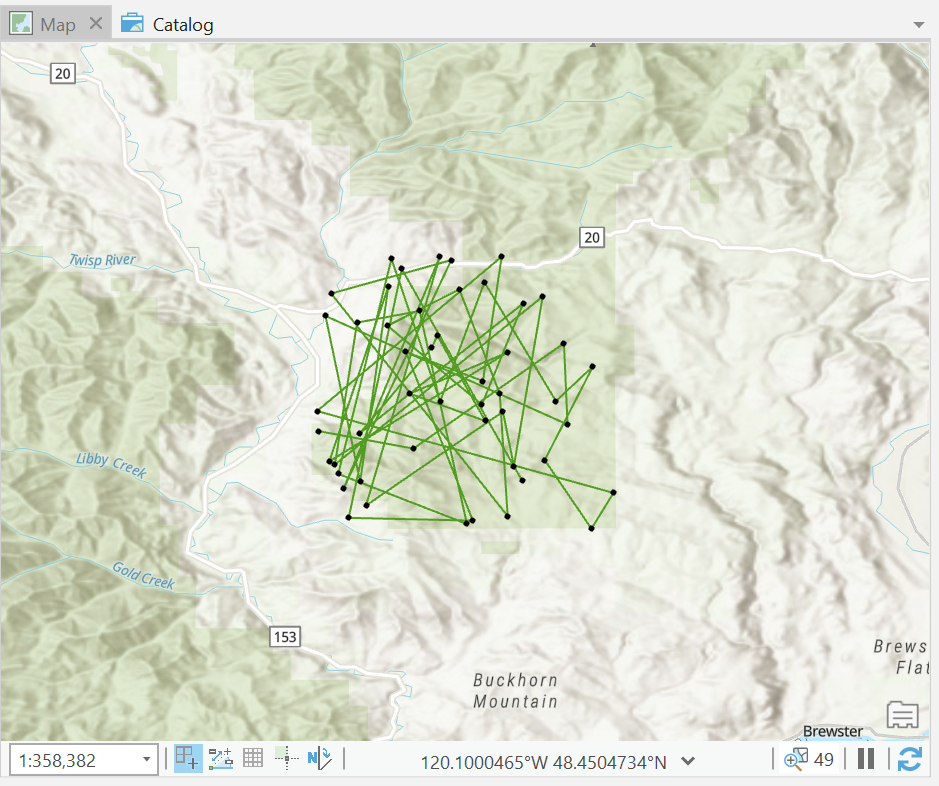
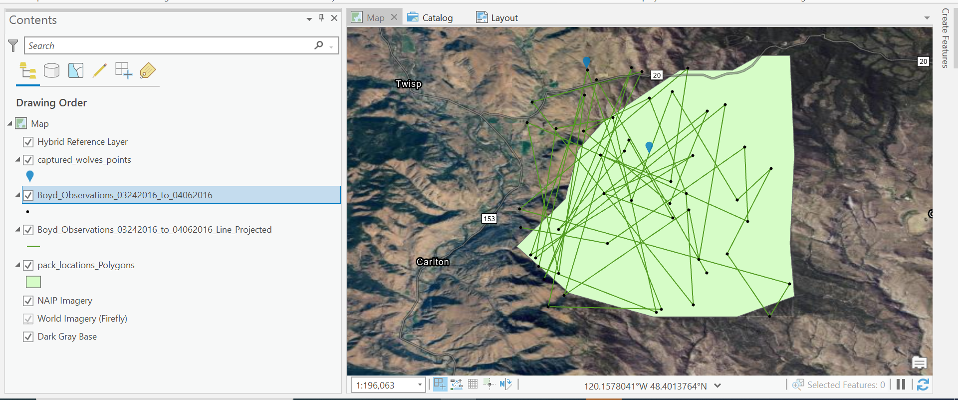
Here’s what my data looks like once its added back to the map.

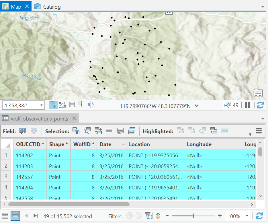
Boyd sure looks like he travels. But these points as they are, don’t really tell us about where he goes, and when. I think that a line, would make sense to see where he went.

Go back to our Geoprocessing Pane and search for Points to Lines.

Once the window opens, notice that there is a little question mark up at the top of the Pane. Click this question mark. This will open the tool documentation.

For this tool, we are wanting to create a line for each wolf and start and order the points based on the date field.

Fill out the fields correctly, save to your geodatabase with a good name and click run!

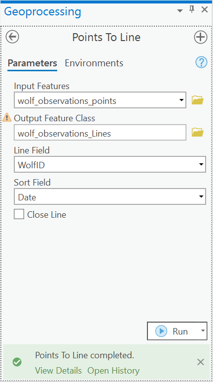
So the result should look something like this.

So now we got some good info for our map. Lets do a couple more field calculations.

So our Line is currently in GCS, which means were are measuring our point locations and lines as (fill in the blank here.)

So we should really think about reprojecting our data here to measure something in terms that we are more familiar with huh.

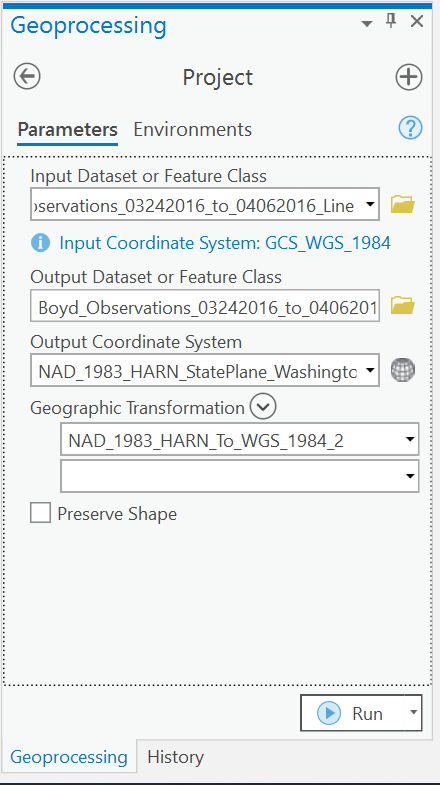
Using the Geoprocessing Pane, lets search for the Project tool.

Lets choose to reproject to Washington State Plane North since we are working with Wildlife Data and Boyd seems to live in the North Cascades.

This changes your data, so again, give it a good name to know what data is in this layer, and why is it different than that last layer we exported.

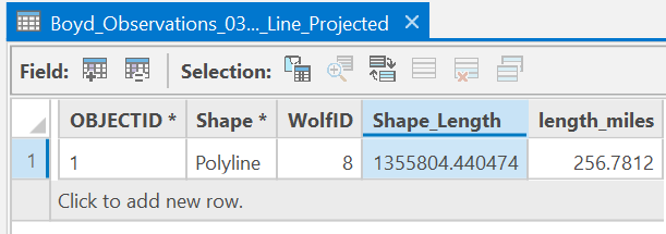
So ArcGIS does this fun thing for us where it automatically calculates the length of our line. If you open the attribute of our new data set, you should see it changed pretty significantly. What unit is this measurement in? And lets convert it into something that makes more sense.

Lets use the field calculator again, and this time, lets create a new field called Length_Miles.

Whatever unit you think this projection uses, convert this number to miles.

This time, you need to choose the right field type. To be able to write your expression, double click the Shape_Length in the fields box. This adds the this a variable in your expression. A now, multiply/divide accordingly to convert these original units to miles.

Something like: !Shape_Length! / your conversion unit

Lets get some more information

Our objective here is that we are going to create a map of Boyds two weeks, and summarize other information about Boyd in a nice page summary.

Lets get the following information about Boyd.

• How many other wolves and what are the names of the wolves in Boyds Pack?
• Who is the oldest and youngest member in this pack?
• Are there any other wolves in the pack that are collared?
• What is the average weight, and health condition of the male wolves that have been captured and are alive in the North Washington Packs? How does this compare to Boyd?
• For the sampled observations, how much time are the wolves spending time inside the pack boundary vs outside the pack boundary (just in terms of observations)? Do you think we need to expand the boundary based on this number?

Using the joins and selction using logical operators, answer these questions. Additionally, for this last question you are going to need to do some spatial logical operators. Try using the Select by Location tool. Also, once you run your queries and get the results, it might be easier to do the summary math outside of ArcGIS.

Lets Map It.

Well now we are getting somewhere. To make this a meaningful map to present our data, we may want to include some more information on our map, include some other features for context and provide labels to make sense of our path.

First, lets change our basemap to something more inviting for wolves.

On the Map tab of the Ribbon, click Basemap, change the Basemap to something that reflects wolf habitat a bit more.

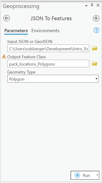
Second, lets try to import our pack locations using the included geojson data.

Use the Geoprocessing pane and search for JSON to Features. Run this tool with our geojson file and the input and the destination as our default.gdb. Run and add the Polygon to your map.

Now lets also show the Capture_Wolves Point Locations for only Boyd. Use a tool to filter the records to only capture locations for Boyd.

Now we are getting somewhere.

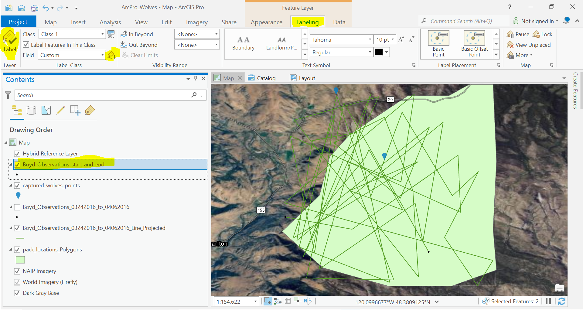
A good map only shows what it needs to, so lets change our symbology to something more appealing, and remove some features to only show whats relevant, say, the start and end dates of our map and where they are.

For Boyds Observations, lets only select the two points assoicated with the start and end of our observation period. Export these features, to your database, and remove the observations from the map.

Click on the new Start_End Date Layer. In the Ribbon, there will be a Tab called Labeling.

Click on the Label Button.

Click on the Expression Button that is in the Label Class section of the Ribbon. This will open a new window. Use Arcdae as the language and in the expression copy and paste the following.

ISOMonth($feature.Date) + '/' + Day($feature.Date)

Use the following format for the lab:

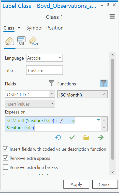
Hit Apply. Your two points should now be labeled with the appropriate Month/Day format.

Now lets change the Symbology of some of our other layers.

We are going to create a Domain to be able to help our data look cleaner.

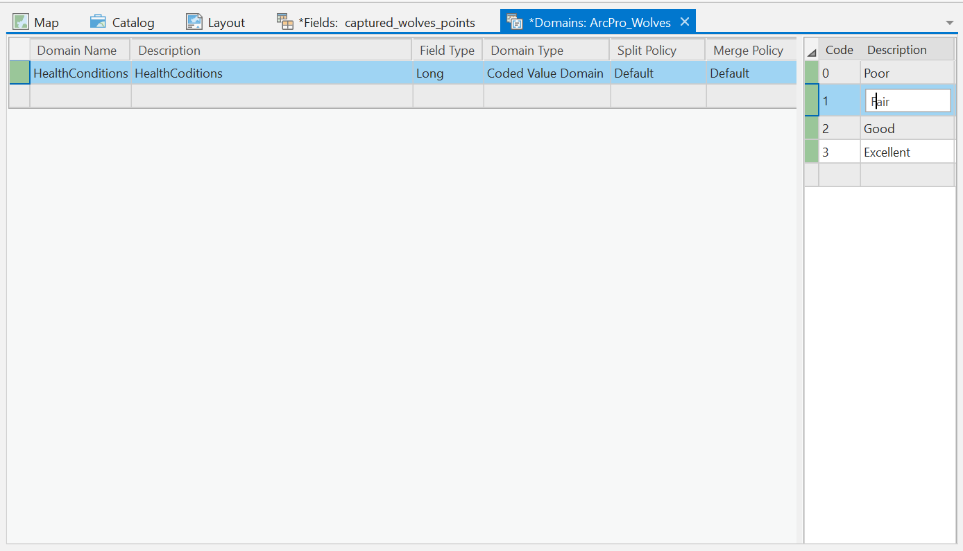
Go to Catalog. Right click our captured_wolves_points layer and select Data Design -> Domains.

This will open a new view.

A domain is a tool which lets us only select a coded value from a field, and populate it with categories from another table. It operates very similarly to a join, however, the field will be resrticted to only the values that are in the domain.

Additionally, it lets us add descriptions for certain codes, and looks up these items automatically for us.

We are going to copy the data from our conditions table into this domain table.

Click the save button in the Ribbon.

And then, we are going to edit the field in our conditions.

Go to Catalog. Right click our captured_wolves_points layer and select Data Design -> Fields.

This will open a new view.

In the Domains column, select the Health Field, it should show you the Domain that we just created above. Select this.

Click save in the Ribbon.

Now in the Map, we can open the Attribute table. See the Health Field now looks up the values in this Domain table to get the correct key. This is especially helpful if you are working with categorical data, and you want to rename your category.

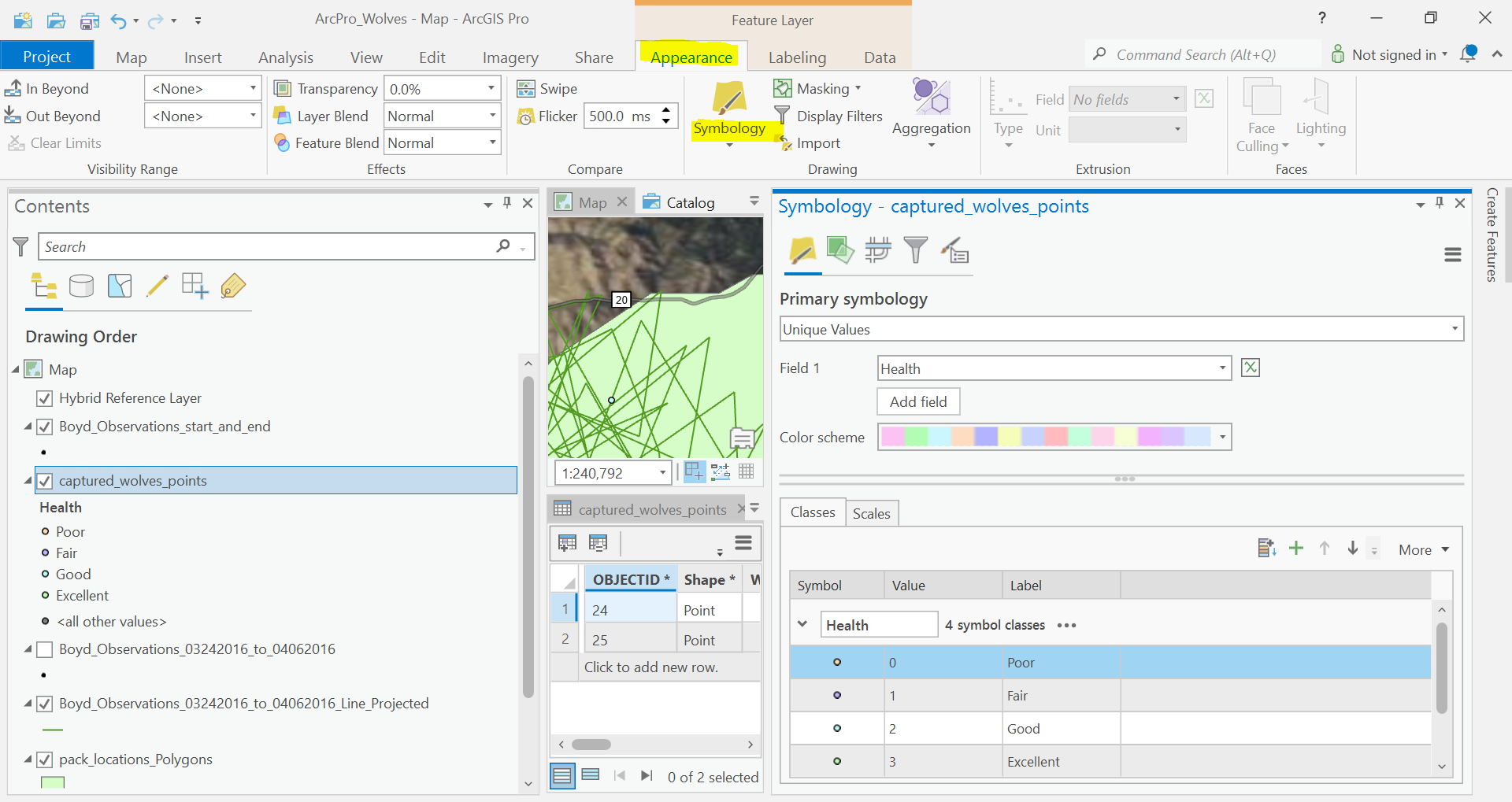
Lets Symboloize our Data with Unique Values using the Health Field.

Click on the Layer in the Contents Pane of the Map View. The Ribbon at the top of the map will show Appearance -> Symbology button.

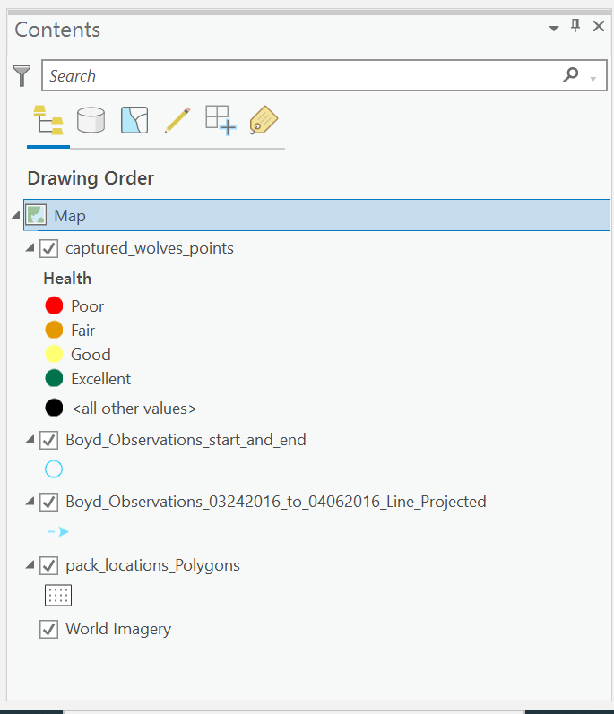
Change the symbology to Unique Values based on the Health field. Change the symbols to something that appeals to you, and can show the difference between the different categories of data.

Lets also repeat our labelling process of this layer, but give some details about the year.

Here is a code that you can use.

'Captured: ' + ISOMonth($feature.Date) + '/' + Day($feature.Date) +'/' + YEAR($feature.Date)

Fianlly, lets repeat for the Transect and the Pack Polygon Layer. Change the Symbology that clearly lets you see what we are communicating in this map. That is, Boyds Travels over a two week date range.

Heres what I chose.

Great. Now lets add our reference matierals.

Put them in locations where it is easy to see them. In the properties for each item, you can change things like the background color so you can overlay items on the map. Mess around here.

Additionally, for the legend, you can rename the items in the map, by renaming the layers in your map frame. Give your layers names that will communicate what the layers are in the map.

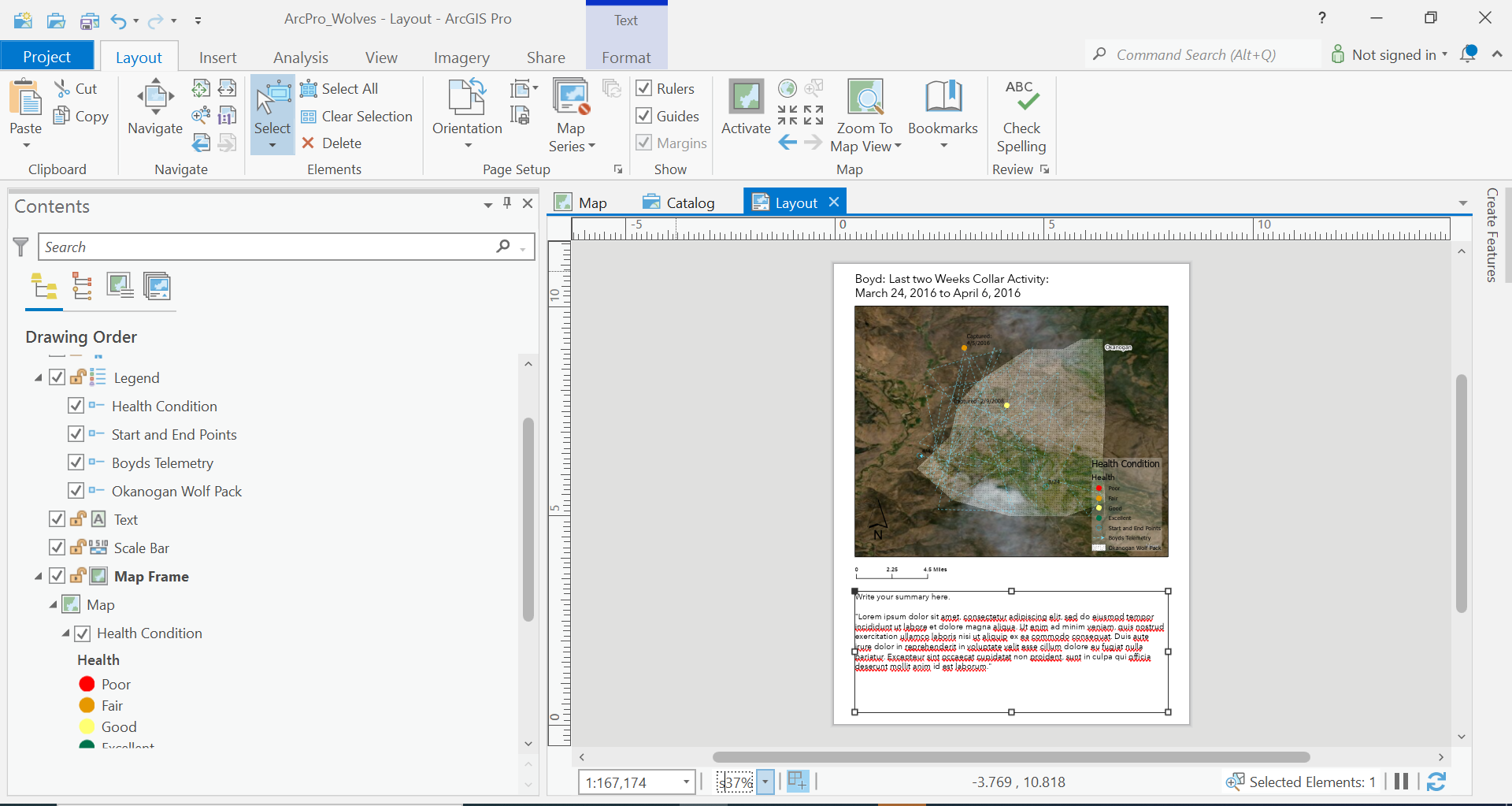
Finally, put a text box at the bottom of the page summarizing the findings that you had from the four questions above.

Compare how Boyd is to the rest of his pack, is he healthy compared to other lone wolfs out there?

Export you map again as a jpg with 150 px resolution. Post to the discussion board for this assignment.

And your Done!!!